
Rules of Inference
(Pt. II)
It is possible to invent a single machine which can be used to compute any computable sequence.
~Alan Turing
Important Concepts
Subderivational Rules
Clarifications
Using subderivational rules might take some getting used to. Students typically are unsure as to what the P's, Q's, and R's are supposed to represent. In addition to the assigned reading in the FYI section (in particular pages 155-163), I hope that this section will clarify some misconceptions.
Let's begin with an important label. The main scope is the far left bar. That is where your derivations begin and end. Whenever you use a subderivation, you should indent a bit. If you were to use a subderivational rule within a subderivational rule, you should indent again. We will eventually see nested subderivations. The main point here is that subderivations must be ended and the derivation must always conclude on the main scope.
While you are building your proof, you are allowed to cite any line above the line you are working on as long as it is on the main scope. If you are working in a subderivation, you are allowed to cite any line above your current line within the subderivation (including the assumption) as well as any line above the line you are working on from the main scope.
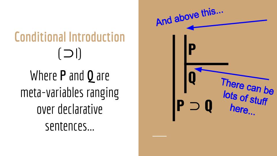
Conditional and biconditional introduction
Let's take a look at conditional introduction (⊃I), which is pictured above. The general idea here is that if you want to couple two sentences of TL with a horseshoe, then all you need to show is that you can move from the antecedent (P) to the consequent (Q) within a subderivation. You place what you want the antecedent to be in the assumption of the subderivation and what you want the consequent to be at the bottom of the subderivation. Then you prove, through the use of the rules of inference, that you can in fact work your way from the assumption of the derivation (the antecedent) to the consequent. Once you've done that, you can end the subderivation and write in your conditional (P ⊃ Q) on the main scope.
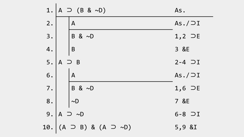
Take a look now at the proof below. Study in particular lines 2-4. This is a conditional introduction in action. During the proof we decided that we wanted to derive "A ⊃ B". The reasoning for this will become clear in the Getting Started (Pt. I) video. Once it has been decided that we want "A ⊃ B", then we have to reason about how to acquire it. Since it is a conditional, it is reasonable to assume that we can derive it using our conditional introduction rule. And so a subderivation is drawn out. Although what you see is the completed subderivation, the method of arriving at that conditional is simply to indent, draw scope lines for the subderivation, place the antecedent of the conditional you want to derive (which in this case is "A") at the top of the subderivation (as an assumption), and place the consequent of the conditional you want to derive (which in this case is "B") at the bottom of the subderivation. Once this setup is complete, your task is to show that you can indeed justify placing the consequent where you did. You will see how this is done in the video. What is important to realize here, however, is that once you've documented your justification of line 4, you can end the subderivation, return to the main scope, and write in your newly derived conditional there. That's how conditional introduction works.
Biconditional introduction is actually very similar to conditional introduction. Essentially, it's just two conditional introductions. This means that two subderivations are required. In the first subderivation, you have to show that, assuming the left part of the biconditional, you can derive the right part; and in the second subderivation, assuming the right part of the biconditional, you have to derive the left part. If you can do this, you can end both subderivations, return to the main scope, and write in your biconditional. You'll see an example of this in the video.
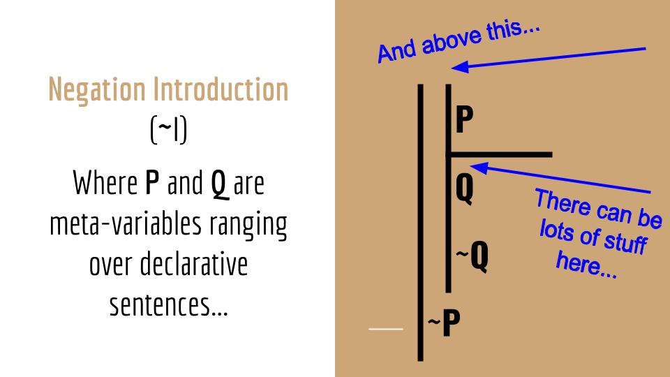
Negation introduction and elimination
Negation introduction and negation elimination work much in the same way. Let's begin with negation introduction. If you've decided that you want the negation of some sentence of TL, basically a sentence of TL plus a tilde to its left, then you should use negation introduction. What you do is: indent, draw scope lines for the subderivation, place the sentence of TL that you want minus the tilde at the top (as the assumption), and the sentence of TL that you want (now including the tilde) after the subderivation on the main scope (see image below). Your task then is to show that you can derive a contradiction "Q" and "~Q" within the subderivation somehow. This contradiction can be composed of any sentence of TL and its negation. For example, it could be "A" and "~A", or "B ∨ (C & ~D)" and "~(B ∨ (C & ~D))", etc. It is once you've established this contradiction that you can end the subderivation and return to the main scope with your newly acquired negated sentence, which should always be the negation of the assumption of that subderivation.
Negation elimination works exactly the same except that your initial assumption should be a negation and the sentence you derive after the subderivation should be the "un-negated" assumption, basically the assumption of the subderivation minus the tilde. In other words, you've eliminated the tilde.
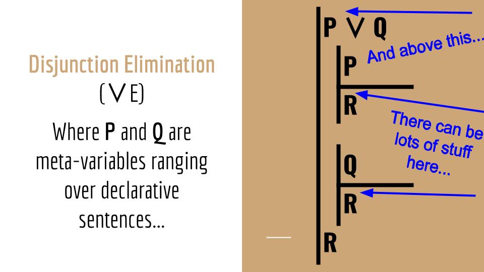
Disjunction elimination
Lastly, there's disjunction elimination. This is probably the most cumbersome of the subderivational rules. It's so cumbersome, in fact, that I usually tell students to only use it as a last resort. Having said that, it is sometimes necessary to use it. It requires the following ingredients: 1. a disjunction (P ∨ Q), a subderivation that goes from the left disjunct (P) to some desired sentence of TL (R), and another subderivation that goes from the right disjunct (Q) to the same desired sentence R. If this can be done, you can conclude with R on the main scope (or whatever scope the disjunction you began with is on).
The intuition behind disjunction elimination is the "damned if you do, damned if you don't" situations we sometimes get ourselves into. Here's an example.
- Either I'm going to my in-laws this weekend or I have to clean the attic.
- If I go to my in-laws, I'll be unhappy.
- If I clean the attic, I'll be unhappy.
- Therefore, I'm going to be unhappy.
Premise 1 is the disjunction. Premise 2 is the first subderivation going from the left disjunct to the sentence to be derived, R. Premise 3 is the second subderivation going from the right disjunct to R. The conclusion is R.
Getting Started (Pt. I)

Storytime!
Although I've been making connections between computer science and logic since day one, in this section we will review some of the most explicit connections between the fields of logic, mathematics, and computer science. The main protagonist in this story is Alan Turing, but we'll have to return to the turn of the 20th century for some context.
In 1900, German mathematician David Hilbert presented a list of 23 unsolved problems in Mathematics at a conference of the International Congress of Mathematicians. Given how influential Hilbert was, mathematicians began their attempts at solving these problems. The problems ranged from relatively simple problems that mathematicians knew the answer to but that hadn't been formally proved all the way to vague and/or extremeley challenging problems. Of note is Hilbert's second problem: the continuing puzzle over whether it could ever be proved that Mathematics as a whole is a logically consistent system. Hilbert believed the answer was yes, and that it could be proved through the building of a logical system, also known as a formal system. More specifically, Hilbert sought to give a finistic proof of the consistency of the axioms of arithmetic.1 His approach was known as logicism.
"Mathematical science is in my opinion an indivisible whole, an organism whose vitality is conditioned upon the connection of its parts. For with all the variety of mathematical knowledge, we are still clearly conscious of the similarity of the logical devices, the relationship of the ideas in mathematics as a whole and the numerous analogies in its different departments. We also notice that, the farther a mathematical theory is developed, the more harmoniously and uniformly does its construction proceed, and unsuspected relations are disclosed between hitherto separate branches of the science. So it happens that, with the extension of mathematics, its organic character is not lost but only manifests itself the more clearly" (from David Hilbert's address to the International Congress of Mathematicians).
As Hilbert was developing his formal systems to try to solve his second problem, he (along with fellow German mathematician Wilhelm Ackermann) proposed a new problem: the Entscheidungsproblem. This problem is simple enough to understand. It asks for an algorithm (i.e., a recipe) that takes as input a statement of a first-order logic (like the kind developed in this course) and answers "Yes" or "No" according to whether the statement is universally valid or not. In other words, the problem asks if there's a program that can tell you whether some argument (written in a formal logical language) is valid or not. Put another (more playful) way, it's asking for a program that can do your logic homework no matter what logic problem I assign you. This problem was posed in 1928. Alan Turing solved it in 1936.

Alan Turing.
Most important for our purposes (as well as for the history of computation) is not the answer to the problem, i.e., whether an algorithm of this sort is possible or not. Rather, what's important is how Turing solved this problem conceptually. Turing solved this problem with what we now call a Turing machine—a simple, abstract computational device intended to help investigate the extent and limitations of what can be computed. Put more simply, Turing developed a concept such that, for any problem that is computable, there exists a Turing machine. If it can be computed, then Turing has an imaginary mechanism that can do the job. Today, Turing machines are considered to be one of the foundational models of computability and (theoretical) computer science (see De Mol 2018; see also this helpful video for more information).
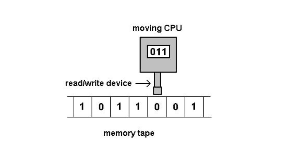
A representation
of a Turing machine.
What was the answer to Hilbert's second problem? Turing proved there cannot exist any algorithm that can solve the Entscheidungsproblem; hence, mathematics will always contain undecidable (as opposed to unknown) propositions.2 This is not to say that Hilbert's challenge was for nothing. It was the great mathematicians Hilbert, Frege, and Russell, and in particular Russell’s theory of types, who attempted to show that mathematics is consistent, that inspired Turing to study mathematics more seriously (see Hodges 2012, chapter 2). And if you value the digital age at all, you will value the work that led up to our present state.
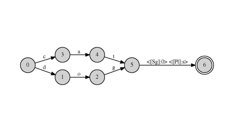
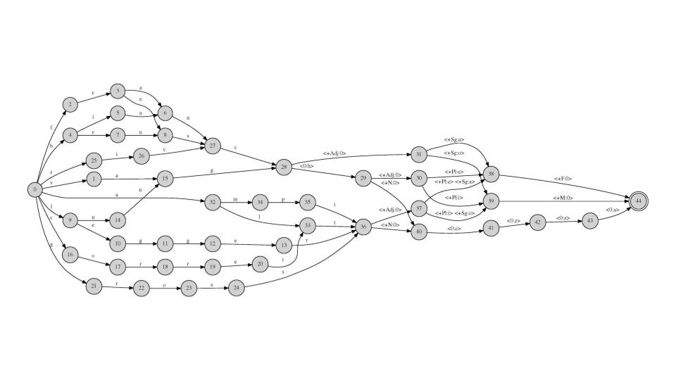
Today, the conceptual descendants of Turing machines are alive and well in all sorts of disciplines, from computational linguistics to artificial intelligence. Shockingly relevant to all of us is that Turing machines can be built to perform basic linguistic tasks mechanically. In fact, the predictive text and spellcheck that are featured in your smart phones use this basic conceptual framework. Pictured below you can see transducers, also known as automatons, used in computational linguistics to, for example, check whether the words "cat" and "dog" are spelled correctly and are in either the singular or plural form. The second transducer explores the relationship between stem, adjective, and nominal forms in Italian.3 And if you study any computational discipline, or one that incorporates computational methods, you too will use Turing machines.
Timeline:
Turing from 1936 to 1950
Intelligent Machines
As the computation revolution was ongoing, Turing began to conceive of computational devices as potentially intelligent. He could not find any defensible reason as to why a machine could not exhibit intelligence. Turing (1950) summarizes his views on the matter. Important for our purposes is an approach to computation that Turing was already pondering.
"Instead of trying to produce a programme to simulate the adult mind, why not rather try to produce one which simulates the child's? If this were then subjected to an appropriate course of education one would obtain the adult brain" (Turing 1950: 456).
When considering the objection that machines can only do what they are programmed to do, Turing had a very interesting insight. Although Turing was brilliant, he knew that the result of his work had in some part to do with his learning growing up. In particular, we've mentioned that the work of Hilbert, Frege, and Russell were very influential. Maybe that's the case with all of us. “Who can be certain that ‘original work’ that [anyone] has done was not simply the growth of the seed planted in him by teaching, or the effect of following well-known general principles" (Turing 1950: 450; interpolation is mine; emphasis added). As the epigraph above shows, Turing was thinking about machine learning...4

Tablet Time!
FYI
Homework!
- Reading: The Logic Book (6e), Chapter 5
-
Note: Read from p. 155-163 and 167-173.
-
Also do problems in sections 5.1.1E (p. 152-155) and 5.1.2E (p. 163-165).
-
Lastly, memorize all rules of inference, both derivational and non-subderivational rules.
-
Note: Your success in this class depends on this.
-
-
Footnotes
1. It was Kurt Gödel who dealt the deathblow to this goal of Hilbert. This was done through Gödel's incompleteness theorem in 1931. The interested student can take a look at the Stanford Encyclopedia of Philosophy's Entry on Gödel’s two incompleteness theorems or this helpful video.
2. Part of the inspiration for Turing's solution came from Gödel's incompleteness theorem (see Footnote 1).
3. Both transducers pictured were made by the instructor, R.C.M. García.
4. According to many AI practitioners (e.g., Lee 2018, Sejnowski 2018), we are in the beginning of the deep learning revolution. Deep learning, a form of machine learning, may prove to be very disruptive economically. We'll have to wait and see (or start preparing).